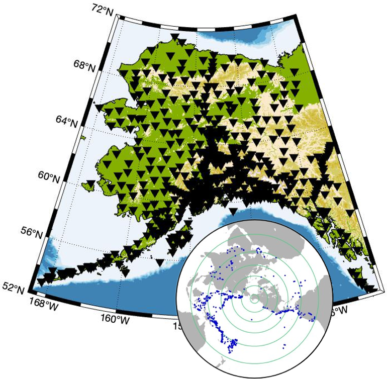
Researchers at UCSB are focusing on measuring seismic attenuation from teleseismic body waves in Alaska. (“Teleseismic” = from earthquakes that are far away from our sensors, “body waves” = seismic waves that dive deep into the Earth’s interior before coming back up to our stations at a steep angle, in contrast to “surface waves” that roll along the Earth’s surface.) Alaska was chosen by the iSTRUM team as a focus site because it provides a useful combination of Earth forcings at different timescales (including glacial and seasonal) as well as excellent seismological coverage. It also includes a large range in physical characteristics (e.g., temperature, melt) associated with the Pacific-North American plate boundary, that make it an ideal natural laboratory for exploring the relationship among state variables, mechanical behavior, and geophysical observables.
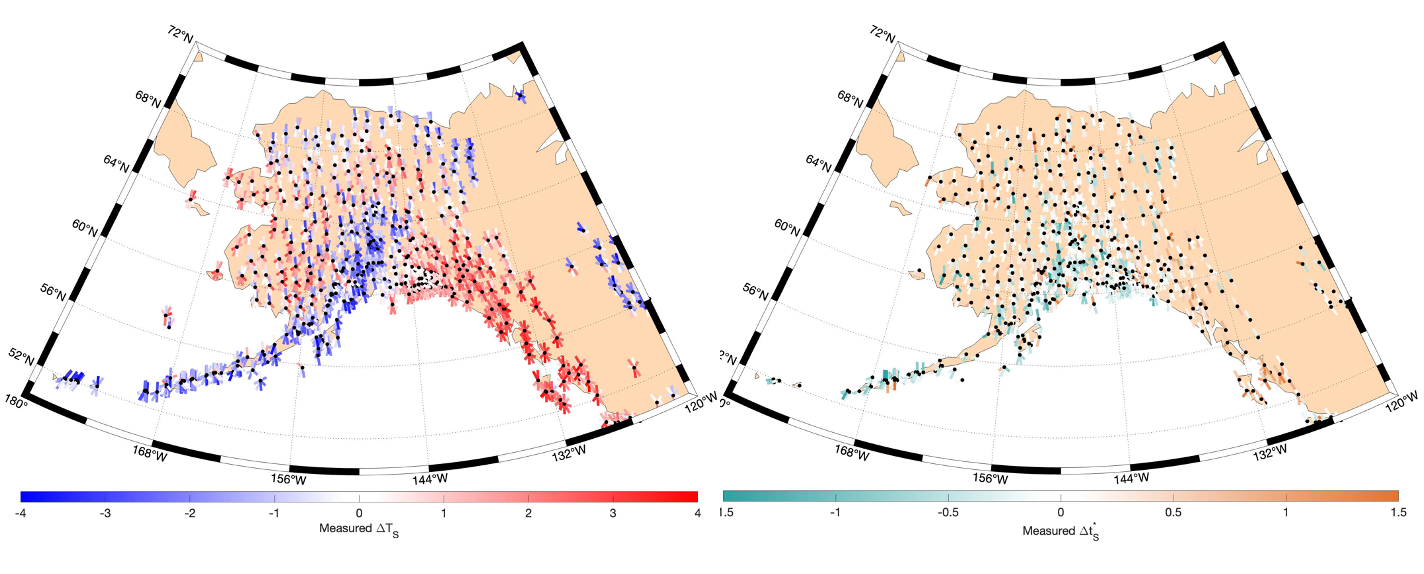
Seismic attenuation, or the rate-of-loss-of-seismic-energy, is quantified by the quality factor, \(Q\), which describes what fraction of a wave’s energy is lost per wave cycle; higher \(Q\) means less attenuation. Since energy is lost each cycle, as the rocks strain one way, then the other, higher frequency waves attenuate more than lower frequency waves (even assuming \(Q\) itself is not frequency dependent; we don’t actually assume this but correct for slight frequency dependence observed in lab settings: \(Q = Q_0 f^{0.27}\)) because for a given distance traveled, higher frequencies have more wave cycles. This is very useful because it predicts a (roughly) linear dependence of wave amplitude as a function of frequency, where the gradient of the amplitude spectrum is proportional to a quantity called \(t^\ast\), which is itself proportional to attenuation (i.e., \(1/Q\)). \(t^\ast\) (pronounced “t-star”) is a canonical measurement of integrated body wave attenuation.
UCSB grad student Cristhian Salas-Pazmino has measured differential \(t^\ast\), the difference between apparent \(t^\ast\) at different stations, for 14,402 P-waves and 11,297 S-waves, as well as differential travel times for 67,671 P-waves and 114,205 S-waves. P-waves have sensitivity to both shear and bulk attenuation and elastic moduli, while S-waves are sensitive only to shear attenuation and modulus.
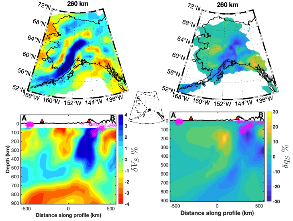
Using these measurements, we have conducted tomographic imaging, building 3-D models of wave speed and attenuation structure beneath the entirety of Alaska. Along the way, we found it necessary to implement significant methodological developments, including multi-frequency travel time measurements for finite-frequency kernels that don’t alias important structural wavelengths, and an iterative inversion for \(\delta(1/Q)\) that allows for significant excursions from a 3-D global starting model. Future imaging improvements will fold in constraints from surface waves (from the Dalton group at Brown) and local body waves (from other collaborators).
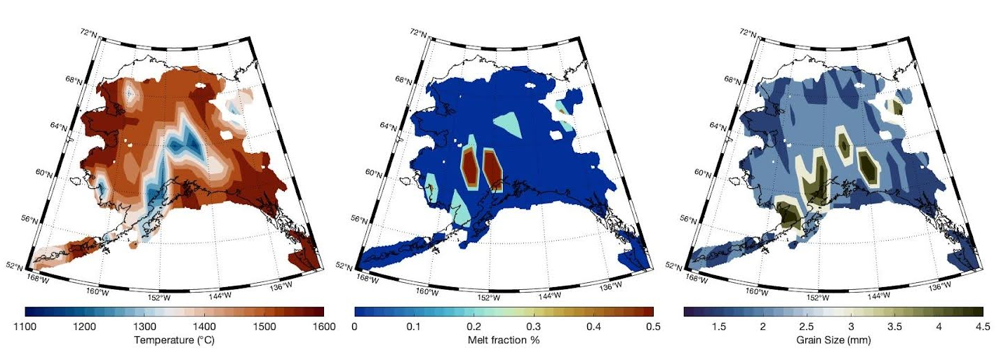
The final stage of our analysis is to interpret our 3-D maps of shear velocity and attenuation for material properties, chiefly temperature, grain size, and melt fraction. We do this using the VBRc (Very Broadband Rheology calculator). We first pre-compute lookup tables that link seismic properties to these state variables, and then use a multi-stage Bayesian approach (also novel) to quantify the most likely material properties. In detail, we first compute posterior probabilities for state variables at each node in our model space with broad priors, then stitch these point-wise distributions together using a smoothing function in 2-D, then re-compute the posteriors using more narrow priors centered on the smoothed maps. The result is a set of probabilistic maps that simultaneously respect both local and regional constraints on these state variables including temperature (\(T\)), melt fraction (\(\phi\)), and grain size (\(d\)),