We are investigating the upper mantle attenuation structure beneath Alaska with Rayleigh waves observed at EarthScope USArray stations. A central goal of the iSTRUM project is to investigate the mantle’s frequency-dependent mechanical response to stress. By using Rayleigh waves in the period range 30-150 seconds, we are providing constraints that probe lower frequencies than the body-wave attenuation study (period range ~1-10 sec) and higher frequencies than probed by ocean tidal loading, hydrological loading, and ice melting. The sensitivity of seismic attenuation to material properties such as temperature, grain size, and partial melt content is complementary to shear wave velocity, making maps of attenuation also useful to improving our understanding of subsurface Earth structure. Alaska provides a natural laboratory to investigate the attenuation signature of a variety of geological settings, including active subduction and volcanism. However, obtaining robust images of attenuation can be challenging, because it is difficult to isolate the attenuation signal in Rayleigh wave amplitude observations. We have been conducting tests with synthetic waveforms to investigate how well Rayleigh wave attenuation can be recovered using an array-based wavefront-tracking approach (Russell & Dalton, 2022).
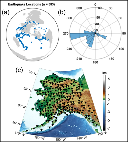
We measured a data set of the amplitudes and travel times of fundamental-mode Rayleigh waves generated by global earthquakes with magnitudes greater than 6 and recorded at 252 stations deployed in Alaska between 2016 and 2021. We have identified three possible sources of error in attenuation results obtained with the wavefront-tracking approach. We designed tests that make use of synthetic waveforms to explore each one.
Overtone Interference#
We seek to measure the attenuation of a fundamental-mode Rayleigh wave, but when an earthquake occurs, it excites not only the fundamental mode but also other seismic phases, including Rayleigh wave overtones. If the overtone arrives at the same time as the fundamental mode, the travel time and amplitude measurements will reflect the interference of the two seismic phases. Hariharan et al. (2020) demonstrated that overtone interference could be minimized by limiting the epicentral distance between earthquake and station to between 20-120 degrees. While we make use of this recommendation to select our earthquake data set, some overtone interference likely remains. To understand what impact such overtone interference would have on attenuation recovery, we conduct a synthetic test in a 1D Earth model with a normal-mode summation method of generating synthetic seismograms.
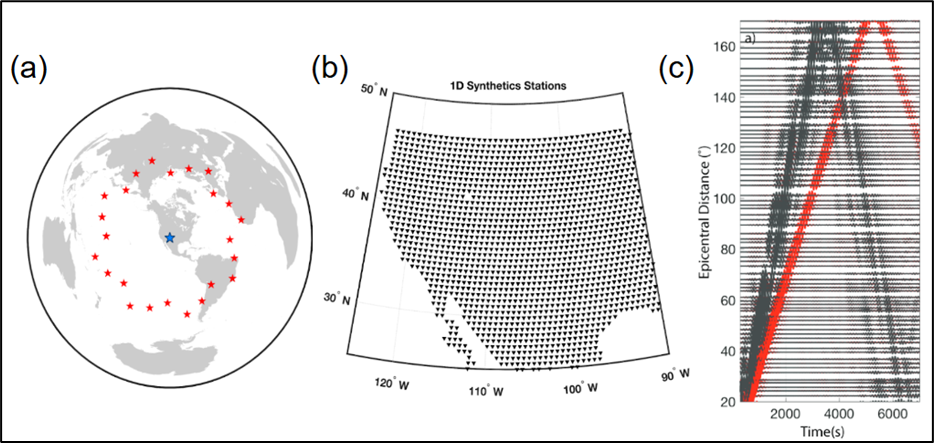
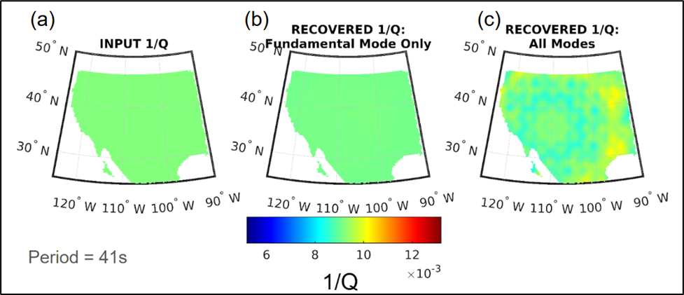
The test set-up is summarized in Figure 2. The test location is the western U.S., and we generalize the results to Alaska. We generate two sets of synthetics, one that contains only the fundamental mode, and one that contains all modes (i.e., the fundamental mode and overtones). The difference in the recovered attenuation between these two synthetic data sets reflects the bias introduced due to overtone interference. Figure 3 shows the result of this test on a color scale set to a conservative estimate of attenuation variations in Alaska. A clear pattern of attenuation artifacts is observed when the synthetic seismograms contain overtones. However, within the context of variations in attenuation we might expect in Alaska, these artifacts should not impact recovery of dominant patterns in attenuation.
Back-azimuthal Coverage#
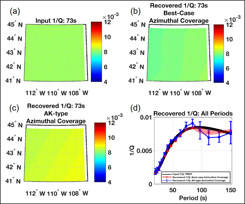
Our wavefront-tracking approach to solving for attenuation maps relies on having uniform azimuthal coverage of earthquakes, i.e., that a seismic station records Rayleigh waves arriving from all directions. However, the azimuthal distribution of earthquakes in our Alaska data set is uneven (Figure 1b). To investigate the uncertainty introduced by imperfect azimuthal coverage, we conduct a synthetic test with waveforms generated using a spectral element method, SPECFEM3D_GLOBE (Komatitsch et al. 2016). We use a 3D Earth model, S40RTS (Ritsema et al. 2011), and a 1D attenuation model, PREM (Dziewonski & Anderson 1981). Twenty-four earthquakes (Figure 4) are distributed evenly around the western U.S., which is the setting for the synthetic test; results are generalized to Alaska. To isolate the impact of uneven azimuthal coverage, we compare the attenuation recovered with this best-case even azimuthal distribution of earthquakes and with an azimuthal distribution that is more characteristic of Alaska.
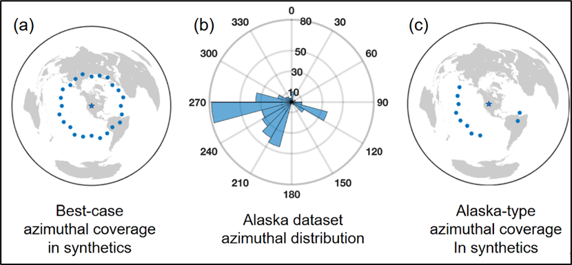
Figure 5 shows the results of this test. We expect to recover a constant value of attenuation across the study area, and we do when the best-case azimuthal coverage is used. However, with the Alaska-type azimuthal coverage, there are artifacts in the recovered attenuation maps. As with the artifacts introduced by overtone interference, these would not entirely overwhelm the signal of large regional attenuation patterns, but they would hamper a robust quantitative interpretation of the results. In Figure 5d, we summarize period-dependent attenuation recovery using the average value calculated from the 2D map at each period. The Alaska-type azimuthal coverage introduces bias into the recovered average attenuation. These large uncertainties would limit an interpretation of attenuation maps in terms of the thermodynamic state of the mantle.
Seismic Station Array Spacing#
Rayleigh wave amplitudes contain contributions not just from attenuation, but also from the earthquake source, the receiver, and elastic focusing during propagation, which is a consequence of wavefronts bending as they propagate through heterogeneous media. Although our wavefront-tracking approach is designed to account for focusing effects on wave amplitudes, the approach is limited by the seismic station array geometry. An array with dense station spacing should be able to capture more wavefield complexity than an array of sparse stations. The EarthScope Transportable Array provided good station coverage across Alaska, with a spacing of around 70 km. However, previous studies of the elastic structure of the subsurface, such as shear wave tomography models, suggest strong focusing effects may be present in the region due to structures such as the subducting Pacific and Yakutat slabs in the south.
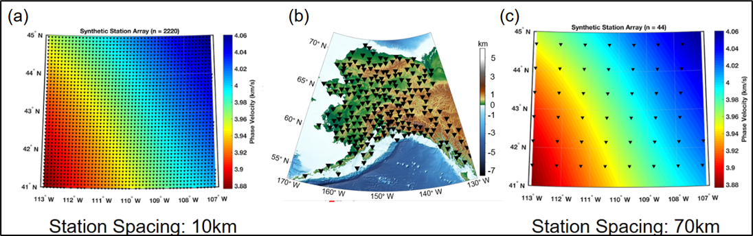
To test the impact of station spacing on attenuation recovery, we set up a test similar to that for azimuthal distribution. We use the best-case earthquake set up (24 events evenly distributed around the western U.S.), but generate two sets of synthetic seismograms, one recorded at an array with 10-km station spacing and one with 70-km spacing (Figure 6).
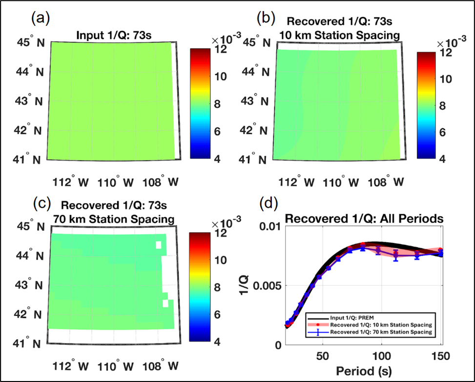
The results are summarized in Figure 7. We observe comparable attenuation recovery and uncertainty with both station array setups. However, we are skeptical that this test tells the whole story. The 3D Earth model used, S40RTS (Ritsema et al., 2011), provides lateral heterogeneity up to spherical harmonic degree 40. This enforces a certain level of smoothness within the velocity model, and regional models of the western U.S. show greater elastic heterogeneity. Further testing is required to determine if the available station array geometry in Alaska can sufficiently recover elastic focusing effects.
References#
- Dziewonski, A.M., Anderson, D.L., 1981. Preliminary reference Earth model. Physics of the Earth and Planetary Interiors 25, 297–356. https://doi.org/10.1016/0031-9201(81)90046-7
- Hariharan, A., Dalton, C.A., Ma, Z., Ekström, G., 2020. Evidence of Overtone Interference in Fundamental‐Mode Rayleigh Wave Phase and Amplitude Measurements. JGR Solid Earth 125, e2019JB018540. https://doi.org/10.1029/2019JB018540
- Komatitsch, D., Xie, Z., Bozdağ, E., Sales de Andrade, E., Peter, D., Liu, Q., Tromp, J., 2016. Anelastic sensitivity kernels with parsimonious storage for adjoint tomography and full waveform inversion. Geophysical Journal International 206, 1467–1478. https://doi.org/10.1093/gji/ggw224
- Ritsema, J., Deuss, A., van Heijst, H.J., Woodhouse, J.H., 2011. S40RTS: a degree-40 shear-velocity model for the mantle from new Rayleigh wave dispersion, teleseismic traveltime and normal-mode splitting function measurements. Geophysical Journal International 184, 1223–1236. https://doi.org/10.1111/j.1365-246X.2010.04884.x
- Russell, J.B., Dalton, C.A., 2022. Rayleigh Wave Attenuation and Amplification Measured at Ocean‐Bottom Seismometer Arrays Using Helmholtz Tomography. JGR Solid Earth 127, e2022JB025174. https://doi.org/10.1029/2022JB025174